Few things in your working life are more guaranteed to cause exasperation than the challenges posed by the need for collaboration with your colleagues. In the context of Microsoft Excel, a frequent source of consternation is sharing a spreadsheet that you have created and refined with great care, only to have the sharer sabotage your efforts (inadvertently or otherwise) by typing over your formula cells, or entering entirely inappropriate data in the wrong location, thereby corrupting your spreadsheet content at the cost of significant time and effort.
Happily, Excel has some simple security features that can help you to prevent this kind of calamity afflicting your spreadsheets. The easiest and simplest of these is the facility of locking cells that you don’t want others to tamper with.
To achieve this, all you need to do is follow these simple steps:
Select the cells, or the range of cells, that you want to be available to other users.
Right-click somewhere over these selected cells and choose Format Cells on the menu
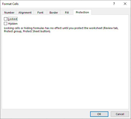
On the right-most tab in this screen called Protection, make sure that the ‘Locked’ check box is un-ticked, hence making sure that all your selected cells are unlocked.

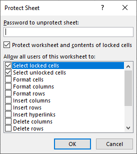
At first encounter, this might seem a trifle counter-intuitive; unlocking cells before you ever lock them. It is important to realise that the default status of all the cells in your worksheet is ‘locked’, which means that if you decide to lock (protect) the entire spreadsheet, theses cells will be locked as well. Once you have thus unlocked the cells that you wish to be available to others, you can then enforce protection on the rest of the spreadsheet via selecting the ‘Protect Sheet’ button on the Review tab. This screen also gives you the option to add another level of security by defining a password to unlock the spreadsheet:

Note that you also have the option in this screen to control how much access other users have to be able to modify or utilise the spreadsheet contents. If you really want to enforce a stringent level of security on your spreadsheet, you might choose to check all the boxes in the lower part of the Protect Sheet screen. Thus, if you then go on to lock the spreadsheet, the other user will be severely constrained in what they can do with your spreadsheet. The main consideration here is really how much confidence you have in the Excel knowledge of your colleagues who might share the spreadsheet. You can, of course, go too far with this form of security, and limit your colleague’s use of the spreadsheet to such an extent that you seriously impede their effectiveness and productivity. As in most things, the wise choice would be to consult with your fellow users first and establish some clear policies for best practice.Once you have defined your password (if required), you can click on OK to finish the process. (You will be required to re-enter your password for confirmation.) Then, if you try and enter or modify the contents of any cells other than those that have unlocked, you will find that you will be unable to so.
To unlock the spreadsheet if required, just select the same ‘Protect Sheet’ button on the Review tab. You will be asked to enter your password to proceed, and if you do so correctly and click on OK, you will be back to square one, with your spreadsheet once again fully accessible to all comers.
This, of course, is just one level of security available in your Excel spreadsheet. If you want to be able to control not only whether or not other users can enter data into specific cells, but exactly what they can enter (i.e. numbers within a particular range, valid department names chosen from a list etc.), you might like to define a validation rule for some ranges within your spreadsheet. Look for more detailed discussion of the validation feature in the near future. In the meantime, check out more advice and info about Excel here.


