Validation in MS Excel

In a recent post, we discussed how you might like to set up some simple protection in your shared spreadsheet, to prevent other users from entering incorrect data into the wrong cells or ranges. But if you are slightly more ambitious with this concept, and are keen to steer your colleagues or any other users along the correct path in their use of your shared spreadsheet, you might choose to take your security to the next level by taking advantage of a feature called validation. In this way, you can not just determine whether or not other users can type into particular cells, but what they can  actually type (i.e. numbers within a particular range, valid department names chosen from a list etc.) Used judiciously, it can be a very effective way to avoid errors or corruption in your spreadsheet that might otherwise undermine your entire efforts.

When using this feature for the first time, a good practice can be to try it out on just one cell, as a test case; you can easily copy or extend your validation settings to a larger or longer range afterwards, an option that we will discuss in more detail below.

First, select the desired cell that you want to use as your test case, and then select ‘Data Validation’ from the Data tab.  If need be, select the leftmost tab called “Settings” in this screen, and select the type of value you are working with from the ‘Allow’ menu, such as ‘Whole number’:
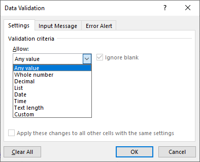
Once you have made this selection, you can define your required the parameters in the lower part of this screen (i.e greater than, less than, between etc.).  This choice alone will define the validation rule for your selected cell; should you now immediately select OK at the foot of this screen, the user would need to follow this rule when entering values into this cell.  Should they err in this process, a warning will appear to inform of their transgression:

The message is rather vague and therefore unhelpful.  You might well choose to customise this message and make it more personalised and enlightening to your fellow user.  You can do so via the ‘’Error Alerts” tab in the same original Data Validation window. Here you can select which icon to display in your warning, give it a suitable title, and then type your desired, appropriate content in the ‘Error Message’ box on the right hand side.

You can provide even more guidance to your users in the same Data Validation screen, via the ‘Input message’ tab.  The input message is a prompt that appears on the screen when you first select the cell with the validation settings defined, and can alert the user, if required, as to what they should be typing to do the right thing and avoid error.  Your Data Validation rule can potentially include all three features:

The essential Settings that define the rule to control any entry in the chosen cell(s).  This is the only mandatory part of this feature.

An Input Message to inform the user of the rule’s requirements

An Error Alert that appears if the user ignores the prompt and makes the error.

It might be tempting to personalise your error message in an attempt to be humorous or derogatory. (For example, “Wrong number, you muppet!”).  This is an impulse best restrained, especially in our current litigious age.  You are on much safer ground with a more neutral, encouraging message. An example might be of the “Bad luck, try again” ilk, with an explanation of why their entry was in error and how they might correct it.

If your validation settings are working for you on your ‘test case’ cell, you can extend the validation to a larger range easily.  All you need to do is to select the range required, along with your test case cell.  Then, you can simply select the same Data Validation option on the Data tab,and you will be presented with the following screen:

Click on Yes, and all of the cells would have the exact same validation rule.

If you acquire confidence in the use of this validation feature, you can be quite creative with it.  For example, if your spreadsheet needs to filled in with some text values, for example department or suburb names, you can use validation to define a list in an interactive menu that your user can choose a valid entry from. Look for a post in the near future on this subject.

Protecting Your Excel Spreadsheet

Few things in your working life are more guaranteed to cause exasperation than the challenges posed by the need for collaboration with your colleagues.  In the context of Microsoft Excel, a frequent source of consternation is sharing a spreadsheet that you have created and refined with great care, only to have the sharer sabotage your efforts (inadvertently or otherwise) by typing over your formula cells, or entering entirely inappropriate data in the wrong location, thereby corrupting your spreadsheet content at the cost of significant time and effort.

Happily, Excel has some simple security features that can help you to prevent this kind of calamity afflicting your spreadsheets.  The easiest and simplest of these is the facility of locking cells that you don’t want others to tamper with.

To achieve this, all you need to do is follow these simple steps:

Select the cells, or the range of cells, that you want to be available to other users.

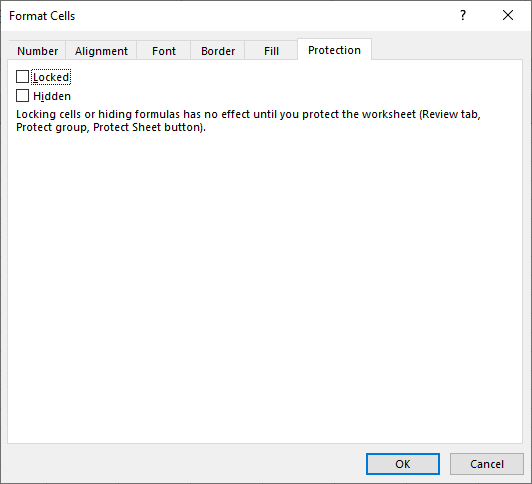
Right-click somewhere over these selected cells and choose Format Cells on the menu

On the right-most tab in this screen called Protection, make sure that the ‘Locked’ check box is un-ticked, hence making sure that all your selected cells are unlocked.

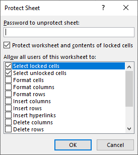
At first encounter, this might seem a trifle counter-intuitive; unlocking cells before you ever lock them.  It is important to realise that the default status of all the cells in your worksheet is ‘locked’, which means that if you decide to lock (protect) the entire spreadsheet, theses cells will be locked as well. Once you have thus unlocked the cells that you wish to be available to others, you can then enforce protection on the rest of the spreadsheet via selecting the ‘Protect Sheet’ button on the Review tab.  This screen also gives you the option to add another level of security by defining a password to unlock the spreadsheet:

Note that you also have the option in this screen to control how much access other users have to be able to modify or utilise the spreadsheet contents. If you really want to enforce a stringent level of security on your spreadsheet, you might choose to check all the boxes in the lower part of the Protect Sheet screen. Thus, if you then go on to lock the spreadsheet, the other user will be severely constrained in what they can do with your spreadsheet. The main consideration here is really how much confidence you have in the Excel knowledge of your colleagues who might share the spreadsheet. You can, of course, go too far with this form of security, and limit your colleague’s use of the spreadsheet to such an extent that you seriously impede their effectiveness and productivity. As in most things, the wise choice would be to consult with your fellow users first and establish some clear policies for best practice.Once you have defined your password (if required), you can click on OK to finish the process. (You will be required to re-enter your password for confirmation.)  Then, if you try and enter or modify the contents of any cells other than those that have unlocked, you will find that you will be unable to so.

To unlock the spreadsheet if required, just select the same ‘Protect Sheet’ button on the Review tab.  You will be asked to enter your password to proceed, and if you do so correctly and click on OK, you will be back to square one, with your spreadsheet once again fully accessible to all comers.

This, of course, is just one level of security available in your Excel spreadsheet.  If you want to be able to control not only whether or not other users can enter data into specific cells, but exactly what they can enter (i.e. numbers within a particular range, valid department names chosen from a list etc.), you might like to define a validation rule for some ranges within your spreadsheet.  Look for more detailed discussion of the validation feature in the near future.  In the meantime, check out more advice and info about Excel here.

Sparklines in MS Excel: What They Are & How to Create Them

One underused, very neglected feature in Excel is sparklines.  When you want to portray a trend in the numbers in your spreadsheet, the best option is to give it a visual dimension, so that it has a much greater impact on the viewer than just showing numbers on a screen (or page).  The obvious avenue to pursue might be to create a chart, and certainly Excel contains a very powerful and elaborate charting facility, that you could employ to serve this need to great effect. However, you may want a simple pictorial representation of the trend that your numbers convey without wanting to invest the time and effort that a full-scale chart might require.

In this case, a sparkline might do just the job that you seek.  The best way to envisage a sparkline is as a miniature chart that occupies no more than a single cell adjacent to the numbers.   The sparklines feature resides on the Insert tab in Excel, just over the halfway point, not far from the charting options.  Perhaps this location, so close to the more commonly used charting creation commands, helps to explain why sparklines tend to be neglected and somewhat underutilised by many Excel users.  (Two of the sparkline options are labelled as ‘line’ and ‘column’ and so, inevitably, they are confused with the charting features that carry the same name and are very nearby on the same ribbon.)

Sparklines are very simple to create. You need only select the first individual cell in the destination range that you intend to populate with sparklines.  Then, go to the Insert tab and locate the Sparklines group, slightly further than halfway along the ribbon.  You have an initial choice of three types of sparkline: line, column or win/loss. (If you are unsure of which type of sparkline will work best, you need not be concerned; you are not “locked in” to your first choice.  You can always revisit your choice at any time, and if need be, change your existing sparkline to any of the other options.)

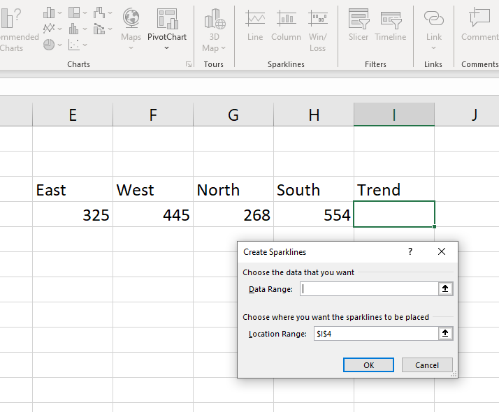
When you select one of the three sparkline options, Excel will ask you for the spreadsheet range that you will base your first sparkline on, and the cell or range you intend to place your sparkline in:

As you can see, the contents of the Location Range box will be the cell you have already chosen.  You just need to place your cursor in the Data Range box, and then select the range that contains the numbers that you wish to use for your sparklines.  In the example above, the Data Range is E4:H4.) Then, select OK and the Location Range cell will display your sparkline result. If you wish to copy the sparkline into an adjacent range of cells, you can use the small green “fill handle” in the lower right corner to easily accomplish this.

To modify your sparkline, you can simply select the cell (or cells) that contain the sparklines, and you will find a Sparklines tab suddenly becomes available at the top of your screen.  The Sparklines tab is a ‘contextual’ tab that only appears when the user selects cells that already contain sparklines.  The attached ribbon presents a range of options that allow you to modify your sparklines, including another chance to choose from the original three sparkline varieties, a style gallery, and the capacity to attach and colour-code markers on various data points on your sparkline.  The options available to you on the sparklines ribbon can be seen on the example below:

Sparklines provide you with a fast and flexible way to add an extra visual dimension to your spreadsheet presentation.

Flash Fill: Data Extraction in MS Excel

In its most recent iterations, Microsoft Excel has changed only minimally, at least as far as the average user is concerned.  Microsoft have only added a few ‘bells and whistles’ to the familiar interface, which have not changed the user’s experience in any fundamental way.  However, one particularly useful enhancement was added to the 2013 version to make the challenge of data extraction both simpler and more intuitive.

Imagine that you are called upon to work with and manage a dataset in an Excel spreadsheet that contains a series of individual names, be they employees, clients, stakeholders or what have you.  The names are contained within a single column, with each consecutive cell containing both the first and last name of the individual concerned, as in the example below:

The problem here lies in the difficulty involved in trying to manage and analyse data in this configuration.  For example, if you want to sort these records in order of the last name, there is no simple way to accomplish this.  With the first and last names combined in the same column in this way, life is much more difficult when it comes to the manipulation and meaningful interpretation of these records.  You really need to separate the first and last names into separate distinct columns to provide you with the flexibility needed in order to facilitate the greater manipulation you desire.

There exist two obvious ways to achieve this.

  • There has long been a feature in Excel called Text to Columns, found a little more than ½ way along the Data ribbon, which exists for the sole purpose of dividing single columns of text into multiple columns of text. This can do the job well, but it requires the user to navigate their way through a series of screens in a wizard to achieve the desired outcome.
  • You can undertake an exhaustive (and quite possibly exhausting) cut and paste operation to create the separate columns as required.  The obvious problem with this is that you may have a significant list of, for example, 100 (or more) names; going the cut-and-paste route could be tedious and long-winded in the extreme.

There must be a better way to achieve this kind of data extraction in a simpler and more intuitive way. Happily, from the 2013 version onwards, there is.

If you go to a blank column adjacent to the list of names and enter a copy of the first name (insert a new blank column if necessary), you can then use the Fill Handle i.e. the little green square in the lower right corner of the cell to copy this name down to the rest of the cells in the column below.  The use of the fill handle in this way will simply copy the contents of the original cell, which is obviously not what you want.

However, if you immediately activate the Autofill Options menu that will appear in the lower right corner of your destination range, you will see that the last choice at the foot of this menu is called Flash Fill.  If you choose this command, Excel will then produce a list of names from the same relative location in the source column, as in the example below:

Flash Fill can also be found in an alternative location on the immediate right of Text to Columns, in the Data Tools group on the Data tab.  The only possible complication with this method of data extraction is the circumstance that the data in the source column does not all conform to the exact same pattern.  The example that I’ve used so far assumes that each cell in the source contains the first name at the start followed by the last name with a space separating the names.  If one or more of the names doesn’t follow the same pattern, Flash Fill is not clever enough to cope with that situation and will not produce a result for these names as intended; you may find that you will be left with a blank row in this location.

However, by and large Flash Fill is a useful addition to the Excel repertoire, and can provide a much simpler and more efficient means of extracting data across a range of different scenarios.  For example, it is often used to extract the individual elements from an address field and hence create separate columns for street, suburb, state, postcode et al.  This example described here merely skims the surface of the applications of Flash Fill in Excel: it can be a most versatile and flexible element in your spreadsheet toolkit.

Excelling at Excel

Excel is Microsoft’s “killer app”, an indispensable tool for spreadsheet users from all walks of life. Explore the posts below, my human friends, if you seek to unlock the true potential of Excel:

Create a growth series of values in Excel

Create your own personal Autofill series in Excel to save yourself time and effort in repetitive typing

Add some pizzazz to your spreadsheets with some conditional formatting

Take your conditional formatting a step further

Perform some clever date arithmetic in Excel

Make an Excel page “very” hidden

A “warp speed” shortcut to create simple charts in Excel

Extract data for easier manipulation with Flash Fill

Create and modify sparklines to add some additional visual impact to your spreadsheet presentation

Safeguard and protect your valuable spreadsheet content from sabotage, inadvertent or otherwise, by protecting your spreadsheet in Excel

Add some Validation rules to your spreadsheet to ensure that your fellow users only input valid, correct data in the appropriate location

Date Arithmetic In MS Excel Made Easy

One very ‘in-demand’ type of calculation in Excel is date arithmetic, which is often an integral part of invoicing or budgeting. You want to display dates that will occur after a given time period in relation to another given date. For example, you might seek to answer a question such as: what will the date be three months from now? And rather than having to manually enter or update the date in question each time, have this calculation built in your spreadsheet via a formula. Here’s how:

Excel’s TODAY function is a simple way of taking today’s date from your computer’s clock and displaying it in a cell in your spreadsheet. All you need to do is type =TODAY() as follows into a cell and press Enter to see the result:

                                =TODAY()

However, the key consideration is that Excel treats all date/time values as numbers, for all calculation purposes, which can complicate your attempt to add another amount to an existing date. For example, if you want to add 3 months on today’s date, you need to be aware that in Excel, the basic unit of a date value is an individual day; which means that, simply adding the number 3 on to today’s date will display the date 3 days from now.  Which would be just fine, if that be your intention. However, to be able to choose which date/time interval to use in your calculation, you need to incorporate other Excel date functions.

You can use functions such as YEAR, MONTH and DAY to break a date value down to its constituent components, and then add your chosen value to the appropriate component.  You can then use another of Excel’s date/time functions, the DATE function, to compile these individual components (year, month and day) into the desired date result. Let’s consider the example below, assuming that cell B3 contains the current date and the adjacent cell C3 contains a number of years. The YEAR function will extract the year from B3 as a separate individual value, and you can then add the required number of years on to this value specifically.  In the result cell, you can then incorporate the YEAR function along with the DAY and MONTH function as parts within the DATE function to calculate the desired result, as seen below:

In this way, you can manipulate date values in Excel to produce the desired type of elapsed time measurements, and this method should produce this result:

Not as simple and intuitive as it might be, but it works!

Conditional Formatting in MS Excel 2: Highlighting Trends

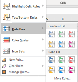
Conditional Formatting in Excel can be used in a variety of ways that can go far beyond simply adding an extra visual emphasis to your important values.  For example, you can use it to give pictorial expression to the trend created by a data series in a spreadsheet. This option can be found further down the main conditional formatting menu, and you can apply it in one of three ways:

  • Coloured Data Bars
  • Colour Scales
  • Icon Sets (symbols)

If, for example, you wanted a visual representation of the differential created by the trend in a series of monthly results;  you can do this by applying your choice of Data Bars to the range in question.

The extent and degree of shading in each cell is determined by the value it contains, compared to the other numbers in the same range.   The higher numbers in the trend exhibit a much higher degree of shading than do the lower ones.  This gives you a method of visually portraying the trend in these numbers, giving your spreadsheet much greater impact than just displaying the bare numbers alone on the screen or page.

If you find that the coloured data bars don’t quite do it for you, there are two other alternatives available on the same menu:

You could go with colour scales, whereby you can represent the same trend with entirely different colours for the higher, lower and in-between numbers. Or you could instead go with Icon Sets and display different symbols such as flags or arrows alongside numbers at different points in the trend.  With any of these choices, you can add a crucial extra visual dimension to your spreadsheet’s presentation.  Which can be particularly useful if you find yourself reporting to a person who sees many spreadsheets in the average day, so much so that they blend together in one homogeneous Excel-y mass.  Conditional formatting is a surefire way of making your spreadsheets stand apart from the crowd!

This assumes ,of course, that you want your spreadsheets to command this sort of attention. And one assumes that you do, at least occasionally, otherwise why would you be reading this post?

Should you wish at a later stage, to edit or modify these conditional formatting rules, you can do so as with any rule – via the Manage Rules option on the Conditional Formatting menu. This dialog box contains both Edit and Delete buttons.

(Bear in mind that you cannot delete conditional formatting via the usual Delete key on your keyboard; this will clear the contents of cells, not the formatting.)

Conditional Formatting in MS Excel

An effective way to that little bit of extra pizz-azz to the presentation of your Excel spreadsheet is conditional formatting. This allows you to emphasis important values and make them stand out visually from the rest of your spreadsheet, as well as making this characteristic part of the overall design of the spreadsheet, rather than just doing manual formatting cell-by-cell after the event. You can define and attach a rule to an entire range, such as a row or column, and thus format whatever values might occupy that range in a standardised way if they meet your chosen criteria.

For example, if you have values that you want to measure against a relevant benchmark or threshold, you can then choose a format such as font, bold, italic, font colour, cell colour, border (or any combination thereof) and those values will accept that format whether they occupy that range currently or in the future.  You need simply to highlight (select) the range in question, and then go to the Home tab and select Conditional Formatting.  If you intend to measure the values against a pre-defined benchmark, the best option is to select Highlight Cell Rules from this menu.  The sub-menu for this option allows you to select a comparison (i.e. Greater Than, Less Than, Between etc). For example, if your threshold is 4000, you can then ascribe a format to values that are below this number via the menu on the right.  See the example below:

This will give cells that contain numbers that are less than 4000 a dark red font colour set against a light red background.

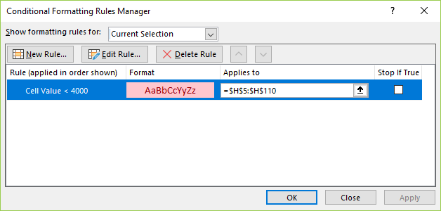
Should you wish to modify this rule, with either or both a different criteria or format, you can do so via the Conditional Formatting Rules Manager, which can be found by selecting Manage Rules… from the foot of the Conditional Formatting menu:

You can modify the rule(s) you have defined via the Edit Rule… button at the top of this dialog box.  Note that you can also delete rules via this dialog and create new rules as well, as an alternative method to doing so via the Conditional formatting menu.

You can create as many different rules for the same range as you wish, and also produce some more elaborate formatting effects by making full use of the variations available on the Conditional Formatting menu. More on this in upcoming posts…

“Warp Speed” Charts in Excel

One of the more impressive and dynamic feature presentation features in MS Excel is charting.  However, in successive versions, the folks at Microsoft have been unable to stop themselves from expanding and complicating Excel’s charting feature to the point where it has become possibly the best exemplar of ‘program bloat’ in the Office family.

For the average Excel user, henceforth, chart creation and modification can be, at best, a time-consuming diversion and, at worst, a confusing and confused labyrinth of excessive choice.  There is, happily, good news for user who is time-poor and seeking to adhere to the sacred principles of KISS.

It is possible to generate a useful chart in Excel via just one keystroke.  You need only select the range of cells in your spreadsheet containing the labels and values that you wish to portray on your chart.  Then, just press the F11 function key on your keyboard and stand back to be amazed!

Excel will instantaneously create a brand new sheet in your workbook, containing a chart based on your selected range of data

A default chart sheet generated in mere seconds with the F11 key

You will immediately have a default 2 dimensional column chart.  Of course, this chart might not be be of a type or format that meets your needs; if so, you can then modify your chart by employing the vast and diverse range of tools to be found on the Chart Tools tab that will appear at the top of the screen whenever your chart window is active.

But if the default chart is enough to meet your needs, very possibly the F11 key is all that you will need. A knowledge of this little-known simple Excel maneuver is also likely to impress your colleagues and workmates, who will likely view you with a new respect and, dare one hope, awe.

For more on charting and other Excel presentation strategies, look for upcoming posts…