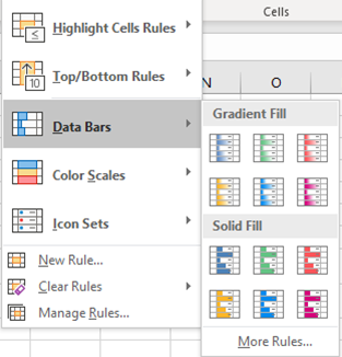
Conditional Formatting in Excel can be used in a variety of ways that can go far beyond simply adding an extra visual emphasis to your important values. For example, you can use it to give pictorial expression to the trend created by a data series in a spreadsheet. This option can be found further down the main conditional formatting menu, and you can apply it in one of three ways:
- Coloured Data Bars
- Colour Scales
- Icon Sets (symbols)
If, for example, you wanted a visual representation of the differential created by the trend in a series of monthly results; you can do this by applying your choice of Data Bars to the range in question.

The extent and degree of shading in each cell is determined by the value it contains, compared to the other numbers in the same range. The higher numbers in the trend exhibit a much higher degree of shading than do the lower ones. This gives you a method of visually portraying the trend in these numbers, giving your spreadsheet much greater impact than just displaying the bare numbers alone on the screen or page.
If you find that the coloured data bars don’t quite do it for you, there are two other alternatives available on the same menu:

You could go with colour scales, whereby you can represent the same trend with entirely different colours for the higher, lower and in-between numbers. Or you could instead go with Icon Sets and display different symbols such as flags or arrows alongside numbers at different points in the trend. With any of these choices, you can add a crucial extra visual dimension to your spreadsheet’s presentation. Which can be particularly useful if you find yourself reporting to a person who sees many spreadsheets in the average day, so much so that they blend together in one homogeneous Excel-y mass. Conditional formatting is a surefire way of making your spreadsheets stand apart from the crowd!
This assumes ,of course, that you want your spreadsheets to command this sort of attention. And one assumes that you do, at least occasionally, otherwise why would you be reading this post?
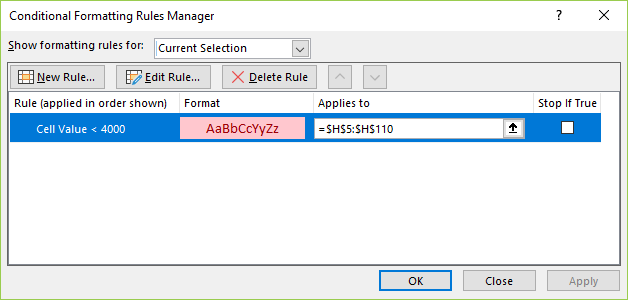
Should you wish at a later stage, to edit or modify these conditional formatting rules, you can do so as with any rule – via the Manage Rules option on the Conditional Formatting menu. This dialog box contains both Edit and Delete buttons.
(Bear in mind that you cannot delete conditional formatting via the usual Delete key on your keyboard; this will clear the contents of cells, not the formatting.)


